Analyzing the Regression Line

Estimating Sigma

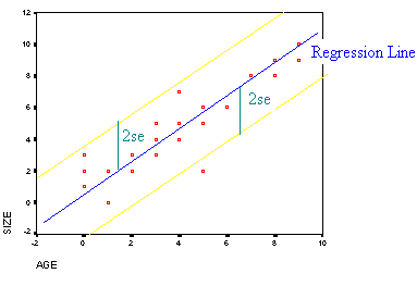
The correlation provides us with an estimate of how linear the data is.  We would also like to know how close the data are to the regression line.  We use a measurement s_e which is a point estimate for the standard deviation for the residuals.  If s_e is large then the points lie far from the line and if it is small then the points are close to the line.  

We have an empirical rule that says that:

        approximately 95% of the points lie within 2s_e of the line.  

 

The mean value for a is a and the mean value for b is b.  Some assumptions that we make on the error e from y = a  +  bx are 

1. e has mean value 0.
   
   

2. e has standard deviation s which does not depend on x.
   
   

3. The distribution of e is normal.
   
   

4. Each of the e's for different x's are independent of one one another.

A point estimate for s² is given by 

SSResid      se2 =                                        n - 2

and the point estimate for s is its square root.

Inferences on the Slope

Suppose that the equation of the regression line calculated from the data is 

        y = a + bx.  

Can we trust this b?  In other words, if the true equation of the regression line is

        y = a + b x,

is b a good point estimate for b?  We can estimate the standard deviation by the formula

The t statistic is

b - b              t =                                        sb   with n - 2 degrees of freedom

We can form a confidence interval for b as

To interpret this confidence for example we can say that we are 95% confident that the true slope of the regression line is between two and three.

If the slope of the regression line is 0 then the regression line is useless.  Hence it is typical to test the hypothesis

        Ho:  b = 0

        Ha:  b 0

We use the t statistic

b - 0       t =                                      sb

and proceed as usual.

Example

Suppose that we have computed the regression line that corresponds to education (years of college) vs. income as

        = 15,000 + 5x

with 200 data points and have 

        s_b = 2

Use 

        a = .05

Then we have 

        Ho:  b = 0

        Ha:  b 0

and 

        t  =  5/2  =  2.5

giving a p-value between .01 and .02.  Since p < a we can reject H₀ and accept H₁ and conclude that the regression line is useful for predicting the income based on college years.  We can make a 95% confidence interval for the slope:

        5 1.96(2) 

or

        [1.08,8.92]

Testing if There is a Correlation

We have talked about the correlation being weak, moderate, or strong; however, with a small sample this may not be reliable.  Smaller samples can produce unreliable results.  Next we will create a hypothesis on whether there is a correlation between the two variables.  If there is no correlation then the correlation coefficient will be 0.  Otherwise it will not be 0.  We can also test to see if there is a positive or negative correlation.  As you may guess, the difference in the test for a correlation, a positive correlation, or a negative correlation will be whether we use a two tailed test, a right tailed test, or a left tailed test.  We will use the Greek letter "r" pronounced "rho" for the population correlation and r for the sample correlation.  The test statistic will be given by

Notice that this is a "t" statistic.  We have

        degrees of freedom  =  n - 2

Notice that the larger the sample size (with the same r), the larger the t value.  Also, a larger r will produce a larger t value.

Example

A study was done to see if there is a positive correlation between  the number of times per month that college students call home and the amount of money that their parents contribute towards their education.  175 students were surveyed and the correlation was found to be 0.18.  What can be said at the 0.05 level of significance?

Solution

First we write down the null and alternative hypotheses:

H₀:  r  =  0

H₁:  r  >  0

We compute the

Since the sample size is large, we can use the normal distribution (z-table) to approximate the P-value.  Notice also that this is a right tailed test so we need to subtract the table value from 1.  We have

        P = 1 - .9920  =  0.008

Since P is less than 0.05, we can conclude that there is a positive correlation between the number of times per month that students call home and the amount of money that their parents contribute towards their education. 

Remark:  We were able to conclude that there is strong statistical evidence of a positive correlation.  On the other hand the correlation of 0.18 is a weak correlation.  Try not to confuse strong evidence to show a correlation with a strong correlation.  Also we can not conclude that calling parents frequently will induce parents to send more money.  We have established correlation, not causation.

Remark:  If the correlation is 0, then so is the slope.  It turns out that the test statistic for the slope is the same as the test statistic for the correlation.  Computers will usually provide the P-value for testing the slope.  This is the same as the P-value for testing the correlation.

Back to the Regression and Nonparametric Home Page

Back to the Elementary Statistics (Math 201) Home Page

Back to the Math Department Home Page

e-mail Questions and Suggestions