Hypothesis Testing for a Proportion and
for a Mean with Unknown Population Standard Deviation
Small Sample Hypothesis Tests For a Normal population
When we have a small sample from a normal population, we use the same method as a large sample except we use the t statistic instead of the z-statistic. Hence, we need to find the degrees of freedom (n - 1) and use the t-table in the back of the book.
Example
Is the temperature required to damage a computer on the average less than 110 degrees? Because of the price of testing, twenty computers were tested to see what minimum temperature will damage the computer. The damaging temperature averaged 109 degrees with a standard deviation of 3 degrees. Assume that the distribution of all computers' damaging temperatures is approximately normal. (use a = .05)
We test the hypothesis
H0: m = 110
H1: m < 110
We compute the t statistic:
![]()
This
is a one tailed test, so we can go to our t-table with 19 degrees of freedom to
find that 
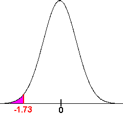
tc = 1.73
Since
-1.49 > -1.73
We see that the test statistic does not fall in the critical region. We fail to reject the null hypothesis and conclude that there is insufficient evidence to suggest that the temperature required to damage a computer on the average less than 110 degrees.
Hypothesis Testing for a Population Proportion
We have seen how to conduct hypothesis tests for a mean. We now turn to proportions. The process is completely analogous, although we will need to use the standard deviation formula for a proportion.
Example
Suppose that you interview 1000 exiting voters about who they voted for governor. Of the 1000 voters, 550 reported that they voted for the democratic candidate. Is there sufficient evidence to suggest that the democratic candidate will win the election at the .01 level?
H0: p =.5
H1: p >.5
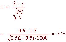
Since it a large sample we can use the central limit theorem to say that
the distribution of proportions is approximately normal. We compute the test
statistic:

Notice that in this formula, we have used the hypothesized proportion rather than the sample proportion. This is because if the null hypothesis is correct, then .5 is the true proportion and we are not making any approximations. We compute the rejection region using the z-table. We find that zc = 2.33.
The picture shows us that 3.16 is in the rejection region. Therefore we reject H0 so can conclude that the democratic candidate will win with a p-value of .0008.
Example
1500 randomly selected pine trees were tested for traces of the Bark
Beetle infestation. It was found that 153 of the trees showed such
traces. Test the hypothesis that more than 10% of the Tahoe trees have
been infested. (Use a 5% level of significance)
Solution
The hypothesis is
H0: p = .1
H1:
p > .1
We have that
![]()
Next we compute the z-score
![]()
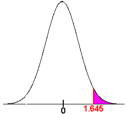
Since we are using a 95% level of significance with a one tailed test, we have zc = 1.645. The rejection region is shown in the picture. We see that 0.26 does not lie in the rejection region, hence we fail to reject the null hypothesis. We say that there is insufficient evidence to make a conclusion about the percentage of infested pines being greater than 10%.
Exercises
-
If 40% of the nation is registered republican. Does the Tahoe environment reflect the national proportion? Test the hypothesis that Tahoe residents differ from the rest of the nation in their affiliation, if of 200 locals surveyed, 75 are registered republican.
-
If 10% of California residents are vegetarians, test the hypothesis that people who gamble are less likely to be vegetarians. If the 120 people polled, 10 claimed to be a vegetarian.
Back to the Hypothesis Testing Home Page
Back to the Elementary Statistics (Math 201) Home Page
Back to the Math Department Home Page
e-mail Questions and Suggestions