Locating and Classifying Local Extrema
Definition of Relative Max and Min
We now extend the definition of relative max and min to functions of two
variables.
|
Definition 1. A function f(x,y) has a relative maximum at (a,b) if there is a d-neighborhood centered at (a,b) such that f(a,b) > f(x,y) 2. There is a relative minimum at (x,y) if f(a,b) < f(x,y) for all (x,y) in the d- neighborhood. |
For differentiable functions of one variable, relative extrema occur at a point
only if the first derivative is zero at that point. A similar statement
holds for functions of two variables, but the gradient replaces the first
derivative.
|
Theorem If f(x,y) has a relative maximum or minimum at a point P, grad f(P) = 0 |
Example
Let
f(x,y) = x2 + xy - 2y + x - 1
then
grad f = <2x + y + 1, x - 2> = 0
so that
x - 2 = 0
or
x = 2
Hence
2(2) + y + 1 = 0
so
y = 5
A possible extrema is (2,-5).
Notice that just as the vanishing of the first derivative does not guarantee a
maximum or a minimum, the vanishing of the gradient does not guarantee a
relative extrema either. But once again, the second derivative comes to
the rescue. We begin by defining a version of the second derivative for
functions of two variables.
|
Definition We call the matrix
the Hessian and its determinant is |

Now we are ready to state the second derivative test for
functions of two variables. This theorem helps us to classify the
critical points as maximum, minimum, or neither. In fact their is a
special type of critical point that is neither a maximum nor a minimum,
called a saddle point. A surface with a saddle point is locally shaped
like a saddle in that front and back go upwards from the critical point
while left and right go downwards from the critical point.
Theorem (Second Derivative Test For Functions of Two Variables)
If grad f = 0 we have the following
|
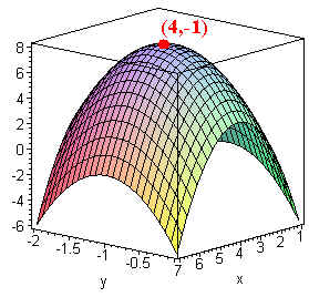
Example:
Let
f(x,y) = -x2 - 5y2 + 8x - 10y - 13
then
grad f = <-2x + 8,
-10y - 10> = 0
at (4, -1)
we have
fxx = -2
fyy = -10 and
fxy = 0
Hence
D = (-2)(-10) - 0 >
0
so f has a relative maximum at (4,-1)
Example: Let
f(x,y) = 4xy - x4 - y4
then
grad f = <4y - 4x3,
4x - 4y3>
We solve:
4y - 4x3 = 0
so that
y = x3
Hence
4x - 4(x3)3
= 0
or
x - x9 = 0
so that
x = 1
or x = 0 or
x = -1
plugging these back into
y = x3
gives us the points
(1,1)
(0,0) and (-1,-1)
We have
fxx
= -12x2 fyy
= -12y2 and
fxy = 4
Hence
D = 144x2y2 - 16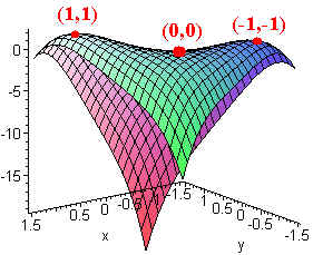
We write the table:
| Point | D | fxx | Type |
| (1,1) | 128 | -12 | Max |
| (0,0) | -16 | 0 | Saddle |
| (-1,-1) | 128 | -12 | Max |
Minimizing Distance
Example
Find the minimum distance from the point (2,1,4) to the plane
x + 2y + z = 5
Solution:
We minimize the square of the distance so that we do not have to deal with messy
roots.
S = (x - 2)2 + (y - 1)2 + (5 - x - 2y - 4)2
We take the gradient and set it equal to 0.
<2(x - 2) - 2(5 - x - 2y - 4), 2(y - 1) - 2(5 - x - 2y - 4)>
= 0
so
2x - 4 - 10 + 2x + 4y + 8 =
0
and
2y - 2 - 10 + 2x + 4y + 8 = 0
simplifying gives
4x + 4y - 6 = 0
and 2x + 6y - 4 = 0
or
2x + 2y - 3 = 0
and 2x + 6y - 4 = 0
subtracting the first from the second, we get:
4y - 1 = 0
so
y = 1/4
Plugging back in to any of the original equations gives
x = 7/4
Finally, we have
s = (7/4 - 2)2 + (1/4 - 1)2 + (5 - 7/4- 2(1/4) -
4)2 = 35/16 = 2.1875
Taking the square root gives that minimum distance of 1.479.
Note that by geometry, this must be the minimum distance, since the minimum
distance is guaranteed to exist.
The Least Squares Regression Line
Example:
Suppose you have three points in the plane and want to find the line
y =
mx + b
that is closest to the points. Then we want to minimize the sum of
the squares of the distances, that is find m and b such that
d12 + d22 +
d32
is minimum. We call the equation
y = mx + b
the least squares regression line. We calculate
d12 + d22 +
d32 = f = (y1 - (mx1+
b))2 + (y2 - (mx2+ b))2 +
(y3 - (mx3+ b))2
To minimize we set
gradf =
<fm, fb> = 0 (Notice that m and
b are the variables)
Taking derivatives gives
fm = 2(y1 - (mx1+
b))(-x1) + 2(y2 - (mx2+
b))(-x2) + 2(y3 - (mx3+
b))(-x3) = 0
and
fb = -2(y1 - (mx1+ b)) -
2(y2 - (mx2+ b)) - 2(y3 -
(mx3+ b)) = 0
We have after dividing by -2
-
x1(y1 - (mx1+ b)) + x2(y2 - (mx2+ b)) + x3(y3 - (mx3+ b)) = 0
-
(y1 - (mx1+ b)) + (y2 - (mx2+ b)) + (y3 - (mx3+ b)) = 0
In S notation, we have
Notice here n = 3 since there are three points. These equations work for an arbitrary number of points.
We can solve to get
and
|
A JAVA Applet that can find the equation and graph the line can be found here.
Exercise: Find the equation of the regression line for
(3,2) (5,1) and (4,3)
Back to the Functions of Several Variables Page
Back to the Math 107 Home Page